

NVIDIA AIBOX 实现单目深度估计
Real-Time Monocular Depth Estimation with NVIDIA AIBOX
Depth perception is a foundational capability for robot localization, mapping, and obstacle avoidance, as well as for environment perception in autonomous driving. A comparison of common depth acquisition approaches is given below:
| Approach | Representative hardware | Main limitations |
|---|---|---|
| Mechanical LiDAR | 16/32-line LiDAR | Starting in the thousand-dollar range; relatively large size and power consumption; contains moving parts |
| Structured light / ToF | RealSense, Kinect | Effective range on the order of 10 m; fails under strong ambient light and on transparent or reflective surfaces |
| Stereo vision | Stereo camera | Depends on baseline calibration; calibration drift over long-term use |
| Monocular depth estimation | Any USB / CSI camera | Output is relative depth; recovering absolute depth from a single frame is an ill-posed problem, so accuracy has a theoretical ceiling |
Rather than relying on geometric constraints, monocular depth estimation uses a convolutional neural network to learn the mapping from monocular cues in a single RGB image — perspective, occlusion, texture gradients, and prior knowledge of object size — to depth, trained in a supervised manner on large-scale image–depth paired datasets such as NYU Depth v2. Its hardware cost and deployment barrier are significantly lower than those of the alternatives: no dedicated sensor, no calibration, and full reuse of an existing camera.

NVIDIA Series AIBOX
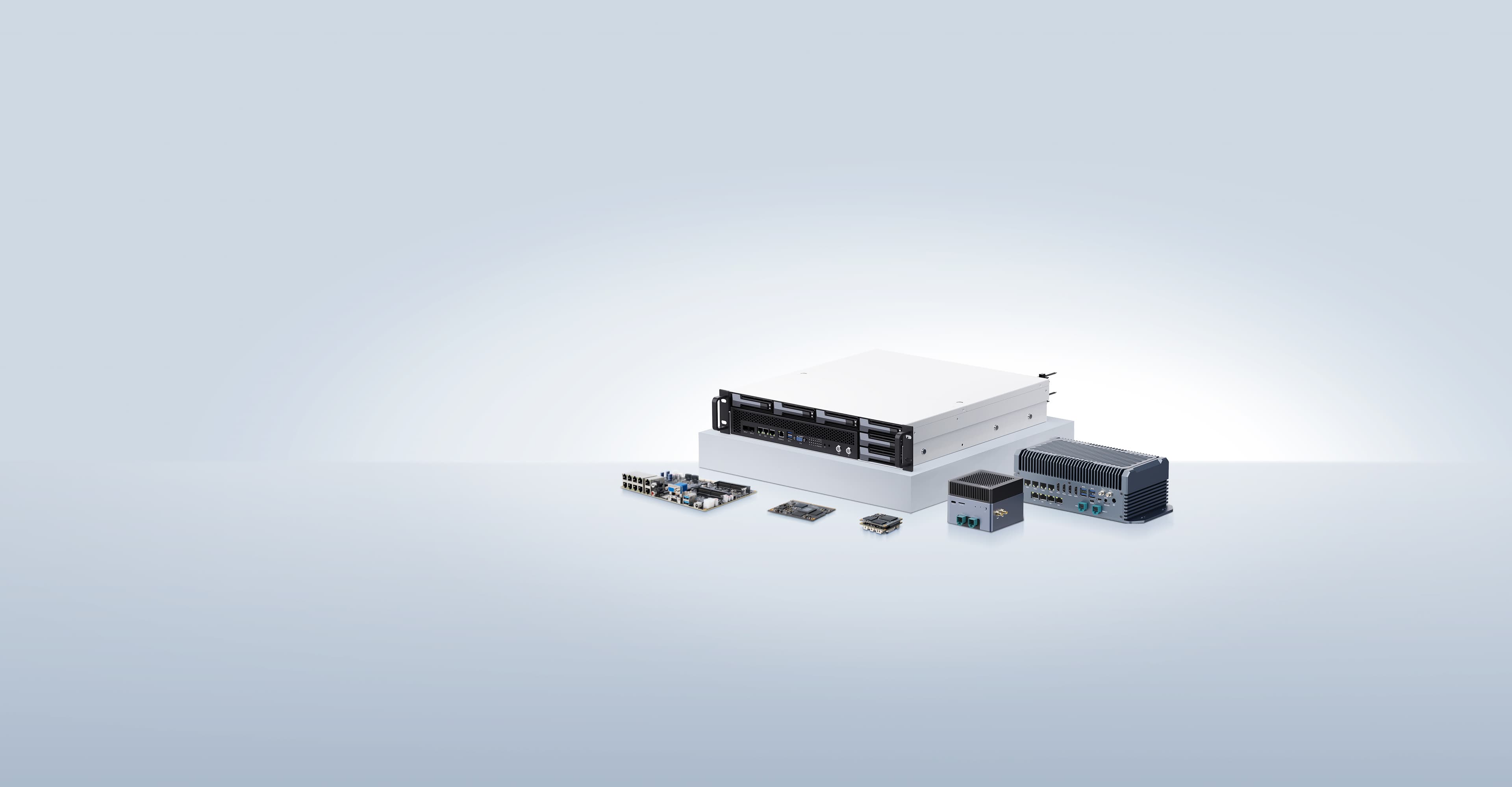
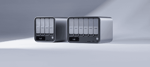
The AIBOX series is powered by original NVIDIA Jetson Orin core modules:
| AIBOX-OrinNX | AIBOX-OrinNano | |
|---|---|---|
| Module | Jetson Orin NX 16GB | Jetson Orin Nano 8GB |
| AI performance | 157 TOPS | 67 TOPS |
| GPU | 1024-core NVIDIA Ampere architecture GPU with 32 Tensor Cores | 1024-core NVIDIA Ampere architecture GPU with 32 Tensor Cores |
| CPU | 8-core Arm Cortex-A78 64-bit CPU 2MB L2 + 4MB L3 | 6-core Arm Cortex-A78 64-bit CPU 1.5MB L2 + 4MB L3 |
| DDR | 16GB 128-bit LPDDR5 102.4GB/s | 8GB 128-bit LPDDR5 68 GB/s |
| HDMI | 4K@60Hz | 4K@30Hz |
For depth estimation workloads, the AIBOX architecture offers three advantages:
- Unified memory. The CPU and GPU share the same physical memory, so there is no cross-bus data copy between video capture, decoding, and inference.
jetson.utils.cudaToNumpy()maps the depth field held in GPU memory directly into a NumPy array that CPU-side business logic can read, eliminating the CPU↔GPU PCIe copy overhead incurred by an x86 + discrete-GPU architecture. - Ample heterogeneous compute headroom. Depth estimation models are purely convolutional and can fully exploit the GPU's CUDA cores and Tensor Cores. AIBOX compute is substantially higher than that of TX2, the experimental platform used in the FastDepth paper — the throughput advantage of the Ampere architecture for FP16/INT8 inference is particularly pronounced — so after running such a model there is still enough compute to concurrently host detection, tracking, and other vision tasks.
- Multi-channel hardware decoding. The NVDEC on AIBOX-OrinNX supports simultaneous hardware decoding of 18 streams of 1080p30 video. Combined with the zero-copy property of unified memory, this makes it possible to build a "multi-stream decode + per-stream monocular depth estimation" pipeline on a single device.
FastDepth Algorithm
FastDepth is a depth estimation network designed for embedded systems; its core strength is the balance it strikes between speed and accuracy.
Network Architecture
FastDepth adopts an encoder–decoder structure implemented as a fully convolutional network (FCN). It takes a 224×224 RGB image as input and outputs a single-channel depth map of the same resolution.

- Encoder: MobileNet. Standard convolutions are replaced by depthwise separable convolutions, which decouple spatial filtering from channel mixing into two separate steps, reducing the computational cost to roughly 1/8–1/9 of a standard convolution.
- Decoder: the core contribution of the paper. Unlike classification tasks, which rely on the encoder alone, depth estimation requires the decoder to progressively restore spatial resolution and produce a dense depth map. Its computation cannot be compressed through layer-wise downsampling the way an encoder's can, so low-latency decoder design is the key difficulty in achieving real-time operation on embedded systems. The FastDepth decoder restores resolution with a combination of nearest-neighbor interpolation + depthwise separable convolution: compared with transposed convolution, this design avoids checkerboard artifacts and further reduces computation, while skip connections fuse features from each encoder stage to preserve high-resolution detail.
Network Pruning
Building on the lightweight architecture, FastDepth further applies channel-level pruning with NetAdapt. NetAdapt is a platform-aware pruning algorithm: it uses per-layer latency measured on the target platform as feedback to iteratively reduce the number of channels in each layer, preserving as much accuracy as possible while satisfying a latency constraint. An analogy from embedded development is trimming functional modules level by level against a MIPS budget: the pruning ratio for each layer is not set by hand, but determined iteratively from measured platform latency.

Implementation in jetson-inference
The depthNet class in the open-source jetson-inference project implements the FastDepth family of models. Two pretrained models are bundled and delivered in ONNX format; on first run, TensorRT compiles an optimized engine for the current hardware:
| Model | Option | Encoder | Characteristics |
|---|---|---|---|
| FCN-Mobilenet | --network=fcn-mobilenet (default) | MobileNet | Fast inference, suitable for real-time streams |
| FCN-ResNet18 | --network=fcn-resnet18 | ResNet18 | Higher accuracy, slightly lower speed |
The model's raw output is a 224×224 single-channel floating-point depth field (relative depth); during visualization it is histogram-equalized and colormap-mapped, then upsampled to the input image resolution.
Deployment
The following steps are executed on the AIBOX factory system; no flashing is required.
Build and Install
sudo nvpmodel -m 0
sudo apt-get update
sudo apt-get install git cmake libpython3-dev python3-numpy

git clone --recursive --depth=1 https://github.com/dusty-nv/jetson-inference
cd jetson-inference

mkdir build
cd build
cmake ../
make -j$(nproc)
sudo make install
sudo ldconfig
Notes:
- The
cmakestage runs theCMakePreBuild.shscript, which downloads pretrained models interactively (including the DepthNet family); simply select the models you need when prompted. Models can also be downloaded later withtools/download-models.sh. - Build output is placed in
jetson-inference/build/aarch64/, with the sample executables under thebin/subdirectory. The Python modules (jetson_inference,jetson_utils) are installed into the system Python path bysudo make install. - If you prefer not to build natively, the project also provides a Docker container workflow (
docker/run.sh); see the official documentation.
Reference: https://github.com/dusty-nv/jetson-inference/blob/master/docs/building-repo-2.md
Run Examples
Process sample images (%i is a wildcard index placeholder):
# C++ sample (under build/aarch64/bin)
$ ./depthnet "images/room_*.jpg" images/test/depth_room_%i.jpg

# Python sample (under python/examples)
$ ./depthnet.py "images/room_*.jpg" images/test/depth_room_%i.jpg
Process a video stream or camera (V4L2 device or MIPI CSI):
$ ./depthnet /dev/video0      # USB camera
$ ./depthnet.py csi://0       # MIPI CSI camera
On the first run of each model, TensorRT compiles an optimized engine for the current hardware; several minutes of build time is normal; the compiled engine is cached to disk, and subsequent runs load at normal speed.
Common Options
| Option | Value | Description |
|---|---|---|
--network | fcn-mobilenet / fcn-resnet18 | Model selection; defaults to fcn-mobilenet |
--visualize | input / depth / input,depth | Combination of content to display |
--depth-size | Float (default 1.0) | Scale of the depth map relative to the input image |
--filter-mode | point / linear | Upsampling interpolation mode |
--colormap | viridis-inverted (default) and others | Colormap scheme |
Raw Depth Field Access and Scale Calibration
The colormapped visualization is intended for intuitive observation only. In engineering applications, the raw depth field should be retrieved through depthNet.GetDepthField() — a 224×224 single-channel floating-point matrix in GPU memory that, once mapped into a NumPy array through unified memory, can be accessed directly from the CPU side:
import jetson.inference
import jetson.utils
import numpy as np

# load mono depth network
net = jetson.inference.depthNet()

# depthNet re-uses the same memory for the depth field,
# so you only need to map it to numpy once (not every frame)
depth_field = net.GetDepthField()
depth_numpy = jetson.utils.cudaToNumpy(depth_field)

print(f"depth field resolution is {depth_field.width}x{depth_field.height}")

while True:
    img = input.Capture()   # assumes a videoSource stream was created
    net.Process(img)

    # wait for GPU to finish before touching the field from CPU
    jetson.utils.cudaDeviceSynchronize()

    # relative depth statistics of the current frame
    min_depth = np.amin(depth_numpy)
    max_depth = np.amax(depth_numpy)
The following semantic constraints must be understood when working with the raw depth field:
- The output is relative depth. The values express depth relationships between regions within the frame; the value range varies with the scene and is not comparable across scenes. Histogram equalization in the colormapped visualization stretches the color band further, so the color scale of the visualization must not be used for distance measurement.
- Metric depth requires scale calibration. Common approaches: solve for the scale factor from a reference object at a known distance in the scene (a person, a shelf, a floor marking), or recover scale by fusing with other sensing modalities such as an IMU or a stereo baseline. This is the essential boundary of monocular solutions relative to stereo, ToF, and LiDAR.
- Resolution and upsampling artifacts. The raw depth field is 224×224; after upsampling to the input resolution, smoothing artifacts are present. Applications with spatial-resolution requirements should evaluate whether this metric meets their needs.